Posts

Summer 2024: Work at ACRE with Purdue Civil Engineering and Agronomy Department

Image
This past summer I had the privilege to work as a UAS pilot at Purdue University's ACRE (Agronomy Center for Research and Education) facility and the subsequent fields that surrounded the area. The fields varied in differing experiments being conducted and monitored on corn, soybean, and sorghum. My role was to continually fly and monitor different fields, collect data and upload data, and maintain a small fleet of various sensors and platforms needed for scientific collection. ACRE fields The flight area was a couple miles West of Purdue University, off of US-52 W. The flights were conducted over a series of both corn and soybean plots throughout the summer. Due to a plethora of conditions including weather and cloud coverage consistency, the flights were largely conducted on a day-to-day basis with the mindset of data collection quality over quantity. Soybean field on 6/7/24 The first couple weeks of data collection was monitoring growth rates of freshly germinated plants. To dem...

StoryMap: Cinematic Data Collection and GIS analysis

Hello all. Despite a lack of posting I have been staying busy within the world of UAS. I would like to share a unique project I composed a few months back. Please feel free to follow the link  here   to view my Esri Storymap. Thanks. Grant

Defining More Features and Buffers

Image
 Features can also be defined measured with other forms of tools and highlighted with buffers. The pairwise buffer tool is helpful in creating zoning areas that can be visually appreciated. Below is a map that has highlighted roads of a flight area at Purdue Wildlife Area. The roads were manually configured using the draw polygon tool. That way, all roads can be accounted for with no error. The roads are still grass features, so the classification wizard querying did earlier would not be accurate, whereas the map above is. Now, I added a 20m buffer from all roads highlighted on the map. This gives you a visualization of the land that is further than 20 meters from all roads. Due, to the road grid pattern being tight, the amount of land is quite small. The buffer feature can also be used for other features. As seen below, I have put a buffer around mostly trees, but in total, all objects that exceed 10 meters in height. Another form of analysis can be found when the same buffers abo...

Object Classification within ArcGIS Pro

Image
 Classifying objects and structures can be very helpful. Whether it be vegetative features, buildings, runoff, rivers, etc. all these features can be accessible through Arc in a variety of ways. Today I will be showing a tools that aid greatly in the classification of features. To begin Esri offers a great step-by-step tutorial on how to use the Classification Wizard, which allows users to create classes of features they want to define, manually outline some of these features, and have the tool automatically define and process the rest. When using the wizard I created two classes to be defined. Those being impervious and pervious features. Above is a neighborhood downloaded through esri that has been partially manually drawn in as impervious (buildings, pavement, etc.) features and pervious (grass, trees, water, etc.) features. However, so much more can be analyzed using the wizard tool. Above is a mission I flew a few weeks back. Using the wizard I was able to classify light veget...

Basic Volumetric Analysis

Image
Volumetric analysis attempts to determine the calculated volume of a pile, area, mining shaft, etc. One can find this by querying out a certain area or polygon, then drawing a base-line so to say that has a minimum floor.  All captured height data determined is measured against that initial floor’s values and one can determine total volume above the plane.  By drawing a polygon around a particular pile and using the extract by mask tool I was able to evaluate the elevations of the pile and then, inserted a volume table beneath the map with total height above 293m msl. A table was made for each different dsm captured at differing dates with coordinate system pixel size (gsd) and minimum and maximum elevation values. Then each was reclassed to smaller sizes (10cm and 100cm). Below are a series of maps with three respective dates and each map with a given date has been resampled to both 10cm and 100cm. Each dsm model has a hill shade with transparency and elevation features have ...

Dredge Pile Raster Extract by Mask and others

Image
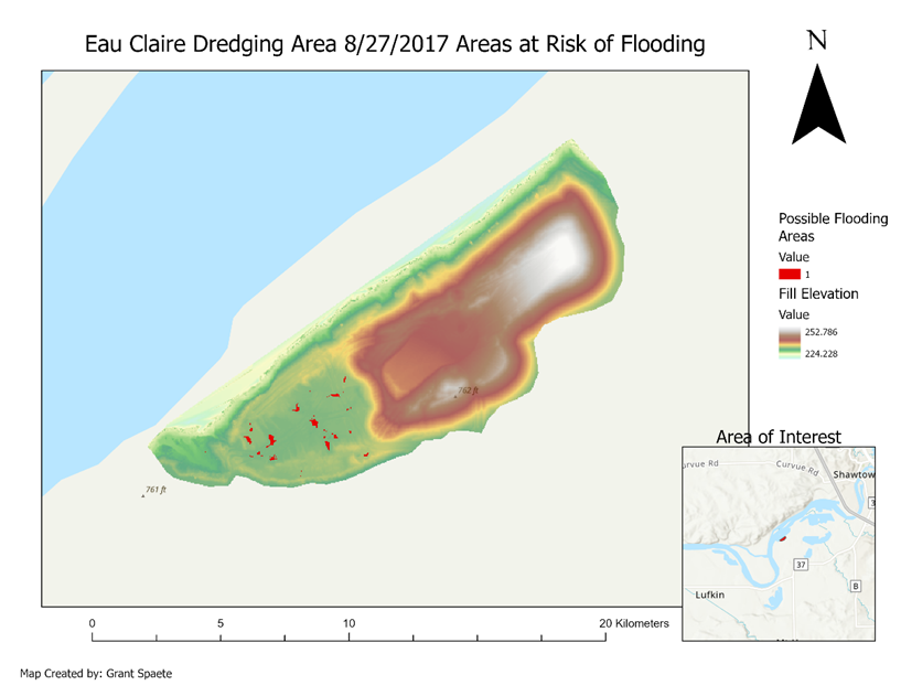
 When using raster data and digital surface models, one can often use many different tools to interpret elevation, slope, and aspect numbers as potential threats to operation or progress being made at a site. For this example I am using a dredging site located in Eau Claire Wisconsin to view many different features that these dsm models can show us.  Over three dates, photos were compiled of this dredging operation, and a dsm was created for each dates so further analysis could be done. Using the extract by mask tool, one can minimize the area of interest as it pertains to a certain elevation, slope, or other value being measured over time. Once, extracted, the model must be resampled in a bilinear manner (by calculating the value of the pixel by averaging the values of the four surrounding pixels) because it is a continuous land feature. Using the map calculator, map values with an elevation of zero were entered to show low spots of the dredging scape, thus, establishing area...

Pix4D Processing and Map Making with Ground Control Points

Image
 The usage of ground control points (GCPs) can be extremely useful when processing data and creating orthomosaic images of an area flown for data analysis. Below I have two instances of processing using GCPs, both of the Purdue Wildlife Area (PWA), and both used for independent and various analyses.  Once in Pix4D, the GCP data collected is set into a file location, and on a spreadsheet, the various figures collected from the GCP during the flight are brought and inserted into Pix4D to begin processing. Initial processing then is selected and let run completely. Make sure correct projection and GCP locations are used before processing is started. Processing varies in time length, but after completion a post processing evaluation should be done.  Next initial processing should be unselected and the next two steps should be run, that being point cloud mesh and lastly the creation of a DSM and orthomosaic model. Once processing is done, locate each GCP location and make sure...